Visualizations can confer useful information about what a network is learning. When building a Convolutional Neural Network to identify objects in images, we might want to be able to interpret the model’s predictions. For example, we might want to explain why the network classifies a particular image as a spaceship. In this post, we look at papers that introduce visualization techniques for CNN-based image classification models.
We first look at Deep Inside Convolutional Networks: Visualising Image Classification Models and Saliency Maps
This paper introduces two ideas for visualizing the workings of the neural network. Both of them require computing of the gradient of the output with respect to the input image.
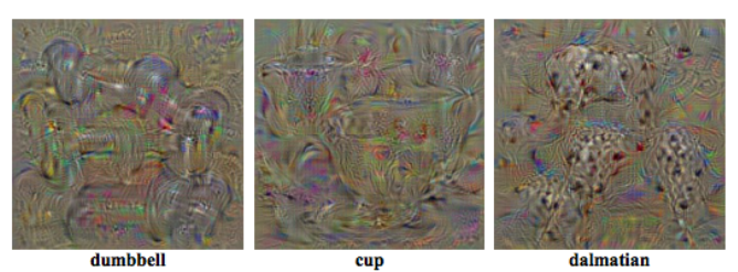
Class Model Visualization: The task here is to generate an image which will best represent a category. Think: what’s the image that looks most like a spaceship to the neural network?. We’re going to find the image $I$ which maximizes the score $S_c(I)$ the network assigns to category $c$; mathematically: $\mathtt{argmax}_I \space S_c(I)$.
Note: the score $S_c(I)$ is the score that the neural network assigns to a class before the softmax, not the probability $P_c = \frac{e^{S_c}}{\sum_c e^{S_c}}$
We can start off with some image $I$, compute the gradient with respect to $I$ using back-propagation, and then use gradient ascent to find a better $I$, repeating the process until we find a locally optimal $I$. This is very similar to the optimization process for training a neural network, but instead of optimizing the weights, we’re optimizing the image, keeping the weights fixed.
 Class model visualizations for 3 different classes. Source: https://arxiv.org/pdf/1312.6034.pdf.
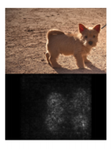
Class Saliency in an Image: The goal here is to find the pixels of an image which contribute most towards a particular classification. Think: what pixels in this image are most important for the neural network to classify it as an image of a spaceship. We’re going to take the derivative of the class score $S_c$ with respect to the input image space $I$, and evaluate at our image $I_0$; mathematically: $\frac{\partial S_c}{\partial I}\bigr\rvert_{I_0}$.
The above derivative gives us a scalar quantity for each of the pixels in the image. Let $w^c_{ij}$ be this quantity at location $(i, j)$ when we’ve used the score for class $c$. We can take the magnitude of these values and then normalize them to get a class saliency map $M_c$ over the image.
$$ M_c(i,j) = \frac{w_{ij}}{\sum_{ij} w_{ij}} $$
 Image-specific Saliency Map shows pixels that are most important for the image being classified as a dog. Source: https://arxiv.org/pdf/1312.6034.pdf.
What’s cool about this? The image specific saliency map can be used for localizing an object of interest (in the above example, we can see where the dog in the image is), and segment it out with the help of a segmentation algorithm. Note that the classification model isn’t trained with object locations; it’s only given (image, category) pairs, but learns to localize: this is called weakly-supervised object localization.
The next paper we’ll look at is Learning Deep Features for Discriminative Localization.
This paper proposes another way to visualize class saliency in images. While the previous paper looks at using back-propagation of the output class score with respect to the input, this paper modifies the network architecture so that the forward propagation can perform both the classification and localization.
The network architecture starts with a sequence of convolutional layers. Passing an image through convolutional layers gives us $k$ feature maps of the image, which are the result of applying learned filters to the image. Each feature map consists of $ i \times j $ activations. Let $f_k(i, j)$ represent the activation at the $(i, j)$th location in feature map $k$.
The score for each class, $S_c$, can then be obtained by summing up the activations within each feature map $\sum_{i,j} f_k(i, j)$, and then taking a weighted average across the feature maps (where the weights $w_k^c$ are learned):
$$ S_c = \sum_k w_k^c \sum_{i, j} f_k(i, j)$$
Aside: Ordinarily, to classify an image, the output of final convolutional layer would be flattened, and then followed by one or more fully connected layers with a softmax activation for categorization. The input size of the fully connected layer would be determined by the size of the input image, making the trained network hard to apply to an image of a different size. The approach taken in this paper avoids that problem, because rather than flattening the feature map, it’s simply summed over, making the approach work with variable-sized feature maps, and therefore with different image sizes. Learn more about this idea, called Global Average Pooling, here.
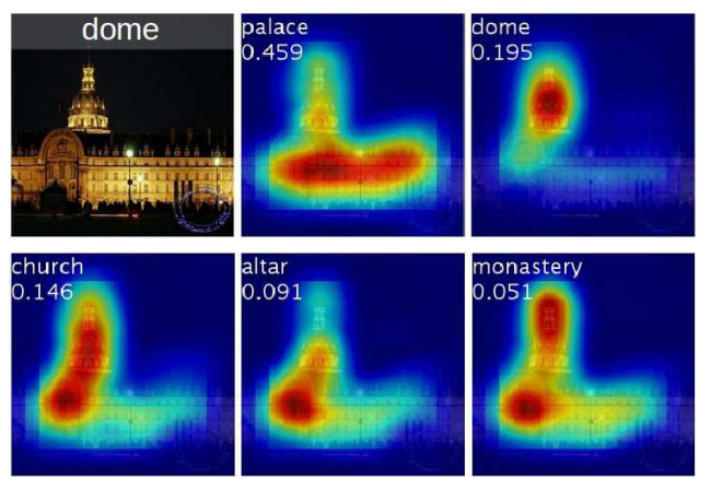
In addition to using this architecture for classification, we can also get a class saliency map, here called class activation map. The idea is to use the learned weight vectors $(w_k^c)$ to take a weighted average of each of the feature maps. Formally:
$$ M_c(i,j) = \sum_k w_k^c f_k(i, j)$$
 Class-activation maps generated for the top-5 predicted classes with their associated class probabilities. Source: https://arxiv.org/pdf/1512.04150.pdf
What’s cool about this? One forward pass can compute both the saliency map and the classification of the image. In fact, we can arrive at the class score from the class activation map $S_c = \sum_{i, j} M_c(i,j)$. Additionally, this method produces visually better maps than those produced by the back-propagation method of the previous paper.