In this post, we provide a walkthrough of how you can run a chest x-ray interpretation model on your own data without writing any code, in just 30 minutes!
CXR Interpretation: Our Journey and Next Frontier
In the Stanford Machine Learning Group and the AIMI center, chest x-ray interpretation, a bread and butter problem for radiologists with vital public health implications, has been one of our primary focus areas.
In late 2017, using the NIH’s Chest X-ray14 dataset released by Xiaosong Wang et al., we built an algorithm (CheXNet) to detect pneumonia and showed that its performance was comparable to radiologists; Luke Oakden-Rayner, Stephen Borstelmann and others reviewed some of the strengths and weaknesses of our setup. In late 2018, we published work showing that an extension of CheXNet (CheXNeXt) could detect upto 10 pathologies at the level of 9 radiologists; at the same time, work by John Zech at al. showed that a reimplementation of CheXNet did generalize well to another institution’s data. In early 2019, we built and released CheXpert, a large dataset of chest x-rays and competition for chest x-ray interpretation (co-released with MIT’s release of MIMIC-CXR by Alistair Johnson et al.), and reported a similar finding of performing comparably to radiologists on some pathologies. Over the past few months, development of chest x-ray interpretation algorithms have been accelerating, with now over 32 models submitted to the CheXpert competition.
Since we published our findings, there have been several groups attempting to reproduce our algorithms (1, 2, 3, 4), and validate them on their own datasets. This is an encouraging signal – before chest x-ray interpretation algorithms can impact clinical care it is important that they be validated on data from other institutions, countries, and patient populations. Validation provides valuable information about the generalizability of the model to different settings, and informs settings in which further development is required for safe and effective use of algorithms.
Making it Easy for Everyone to Validate Our Models With the Help of Codalab.
We set ourselves the challenge of making it as easy as possible for everyone to use our chest x-ray algorithm for validation on external data. Running an algorithm on a new dataset is traditionally a challenging and tedious task, usually requiring computer science expertise, and patience to work through a lot of installation setup. Computer science practitioners are well aware that even when the code is open-sourced, it takes a lot of trial and error to work through installation if the dependencies are not cross-platform, or worse, if they haven’t been specified. Deep learning practice can be even more challenging: local installation is hard because the models may not even fit in local memory. In the remainder of this post, we provide a walkthrough of how you can run a chest x-ray interpretation model on your own data without writing any code, in just 30 minutes!
Walkthrough of Validating CheXpert model on your own data
*For this walkthrough, you don’t need any coding experience. You also don’t need any data: we’ll provide you data example we use for this walkthrough.
We had three of our colleagues go through this walkthrough, including two radiologists, and it took them 21.5 minutes on average using the example dataset.
If you don’t have a dataset right now, download the data we’ve generated, and skip to the next section.
How to Set Up Your Data: Formatting and Organization
If you’re coming in with your own data, this section will help you transform it to the right format.
In this section, we’re going to get your data into a format that the algorithm expects. There will be three things we’ll need: a folder containing x-ray images, a file containing a list of images to be passed into the algorithm, and a file containing information about the ground truth for each of the studies.
For the purposes of this walkthrough, we’ve compiled a dataset of google images of chest x-rays. We constructed this dataset of 96 images by googling for 5 pathologies (Cardiomegaly, Edema, Consolidation, Atelectasis, and Pleural Effusion) on Google Image search and also the Normal category. The first 16 image results judged to not have any annotations on them were chosen to be included, and converted to grayscale. There was no verification of the ground truth performed; this is just a fun dataset that we can share for this tutorial.
Image Directory
The first thing we’ll need is a folder containing all the images in the dataset. We’ll be organizing these images in a very specific format: we recommend that you follow the details closely.
If you’re using the example dataset provided, all the data will already be in the right format, and you can skip to the next section.
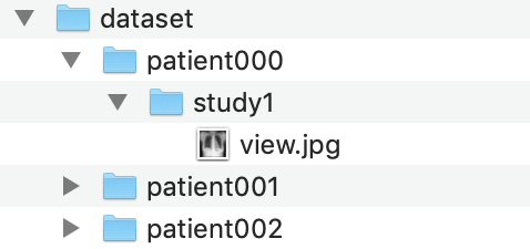 Example image directory
The folder should be structured in the following way:
- The folder should be named ‘dataset’.
- Inside ‘dataset’, there should be folders for every patient (example: patient001).
- Insider every patient folder, there should be a study folder. Each study can have a different ground truth. (example: study1) In our example, we only have one study per patient, but there can be multiple
- Inside every study folder, there should be images (JPG format, ending in .jpg). In our example, we have one image per study, but you might have a frontal and a lateral view.
Finally, this ‘dataset’ folder should be zipped into a file called ‘dataset.zip’. We will use this zip file shortly.
Image Path List
The second thing we’ll need is a file containing the paths of all images we’re running through the algorithm. This file will be in a CSV (spreadsheet) format, which can be generated by Microsoft Excel’s ‘save as’ function.
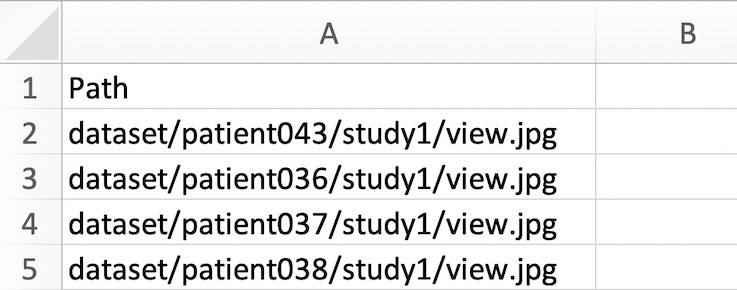 image_paths.csv file
The CSV file should have the following structure:
- The file should contain only one column, with the top row as ‘Path’, and a list of image paths in subsequent rows.
- The image paths must have the format dataset/{patient_name}/{study_name}/{image_name}.jpg
This CSV should be saved with the name ‘image_paths.csv’.
Ground Truth
The third and final thing we’ll need is a file specifying the ground truth for each study. This file will also be in a CSV (spreadsheet) format.
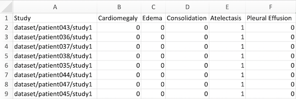 ground_truths.csv file
This CSV file should have the following structure:
- Have 6 columns in total, with the first row containing ‘Study’, followed by the 5 pathologies the algorithm produces outputs for: Cardiomegaly, Edema, Consolidation, Atelectasis, and Pleural Effusion. Our algorithm does not currently support more than these pathologies.
- The paths (in the first column) should have the format ‘dataset/{patient_name}/{study_name}’. Note that these are paths to the studies, not to the images, different from image_paths.csv, which specifies the filenames, while this file specifies the studies. Remember that a study can contain multiple images, but only has one ground truth.
- The values for the ground truth should be 1 or 0, denoting the presence or absence of the pathology.
This CSV file should be saved with the name ‘ground_truths.csv’.
Recommendations For Setting Up Your Data
Ground Truth: Try to set as strong a ground truth as possible on your data. In our previous setups, we’ve used the majority vote of multiple radiologists as the ground truth; others use CT confirmations when possible. A strong ground truth sets the best possible assessment of the model on the data.
Sample size: Aim for as large a validation set as possible. We’ve used the heuristic that the prevalence for each of the pathologies be at least 30 studies.
Images: We recommend that the input images be close to square, and grayscale (the r,g, and b values should be the same), and that images be smaller than 500x500, since the model will downsample them to 320x320 during training.
Running the CheXpert model on your data
We will now run through how you can run the CheXpert model we’ve pre-trained on Stanford data on the dataset you’ve prepared. If you’re using our example data, now’s a good time to download it if you haven’t already At the end of this section, you’ll be able to see the Area Under the Curve (AUC) metric of the model for the 5 tasks on your data (or the example data).
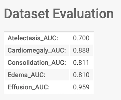 The final output we'll work towards
Creating An Account on Codalab.
We’ll be using the Codalab platform for running the model on your data. CodaLab is an online platform for collaborative and reproducible computational research, developed by Percy Liang at Stanford. The platform has an interface for running commands, using which you will upload your data and run the Chexpert model.
First, we’ll create an account on Codalab:
- Go to Codalab Worksheets and click “Sign Up” in the top-right corner.
- Fill out the subsequent form.
- A verification email will be sent to the email address you used to sign up. When you open it, there will be a link to follow in order to verify your account.
- After verifying your account, sign in again.
- Click on the My Dashboard Link at the top.
Uploading the data on Codalab
We will create a worksheet to organize and setup the running of the model on our data, beginning with uploading the data.
Now, click on ‘New Worksheet’ on the right sidebar.
 New Worksheet
It should prompt you to enter a name for the worksheet.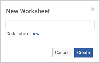 New Worksheet Name
Click on the ‘Upload’ button in the sidebar: Upload
Upload dataset.zip first (dataset.zip is the zip file within the folder you downloaded). In a few seconds, you should see a table with a row added on the left side of the page (refresh the page if you don’t). Then upload image_paths.csv, and then ground_truths.csv, one by one.
If you uploaded the wrong file, you can simply right click on the new row that has been added to the left of the page, and select ‘Remove Bundle Permanently’.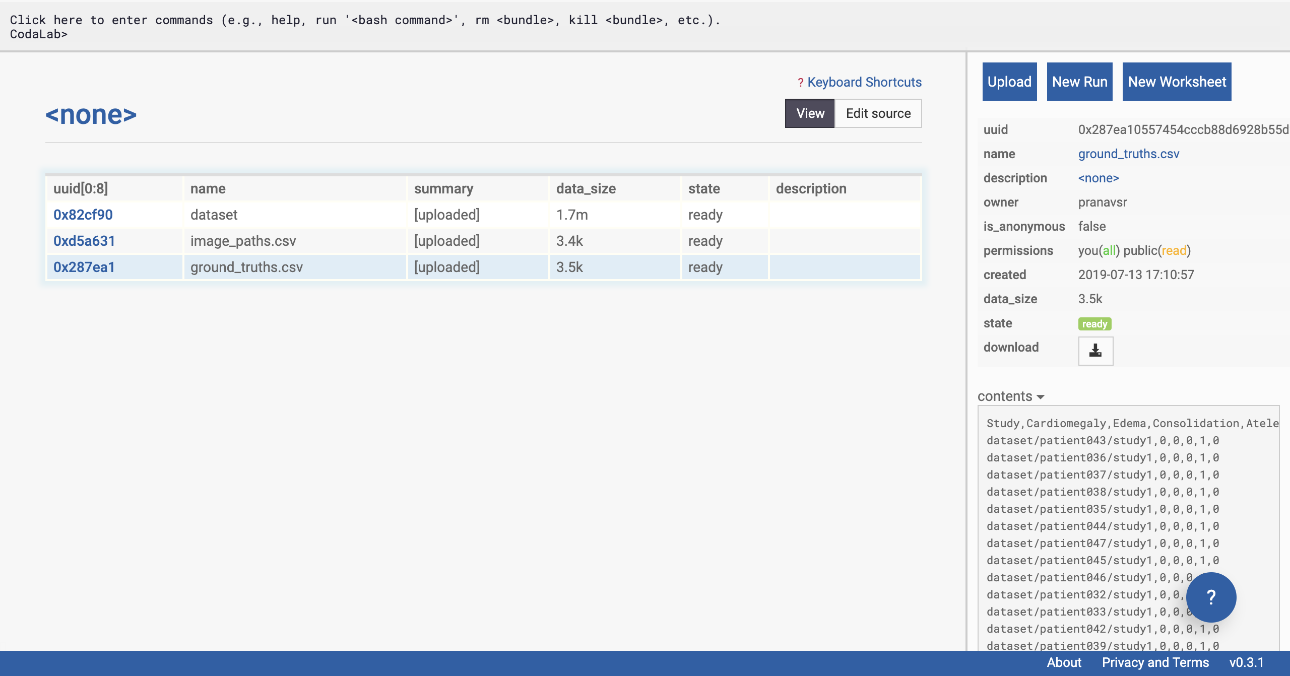 All Files Are Uploaded
Running the CheXPert Model on the Uploaded Data
Now that the data is in place, we’re going to run the CheXPert model on it.
We’re going to first click on the gray pane at the top of the webpage (might contain ‘Codalab>’).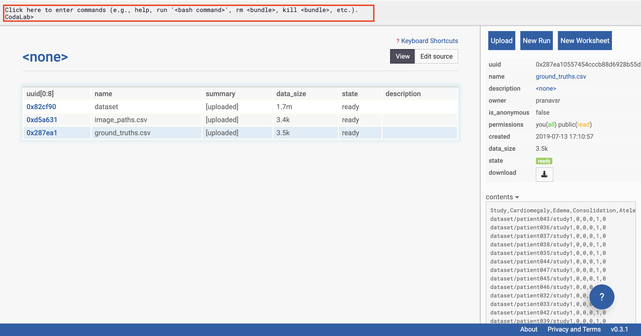 Click the Command Pane
Once we have clicked on the commands pane, the pane will expand. Copy the following command into the pane, and press enter:
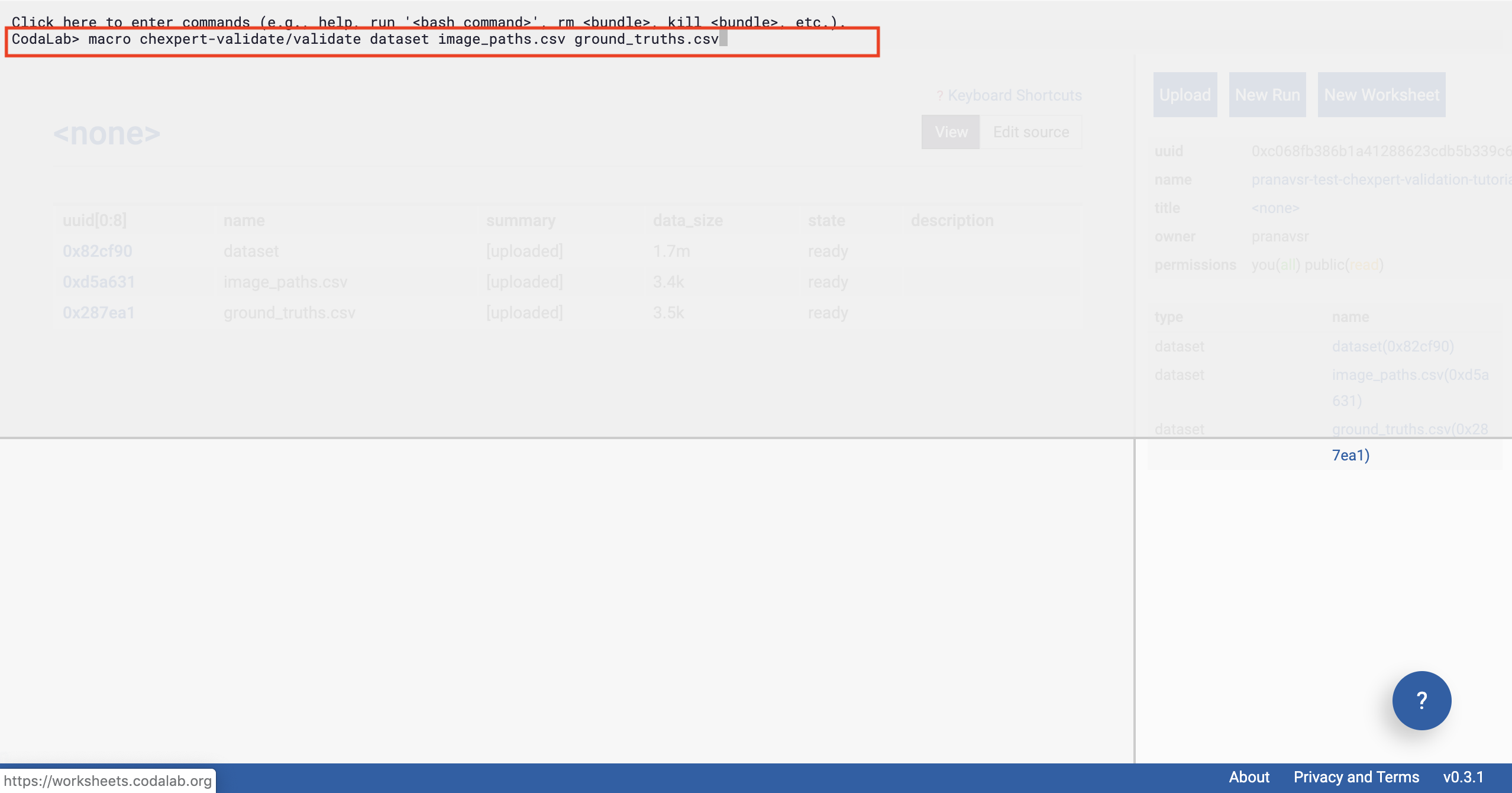 Enter the Command
In a second or two, you should see some output from the interface (after you’ve pressed enter).
Then click outside the pane (shown in figure below).
Congratulations, you’ve already kicked off the run of the model on the data in just one line.
There’s a lot of magic behind the scenes that Codalab performs to make this possible in just one line. Behind the scenes, the CheXpert model is being downloaded onto a remote machine with a GPU instance, on which a Docker container will be set up soon. This Docker container loads all the required dependencies to run the exact environment that the model needs.
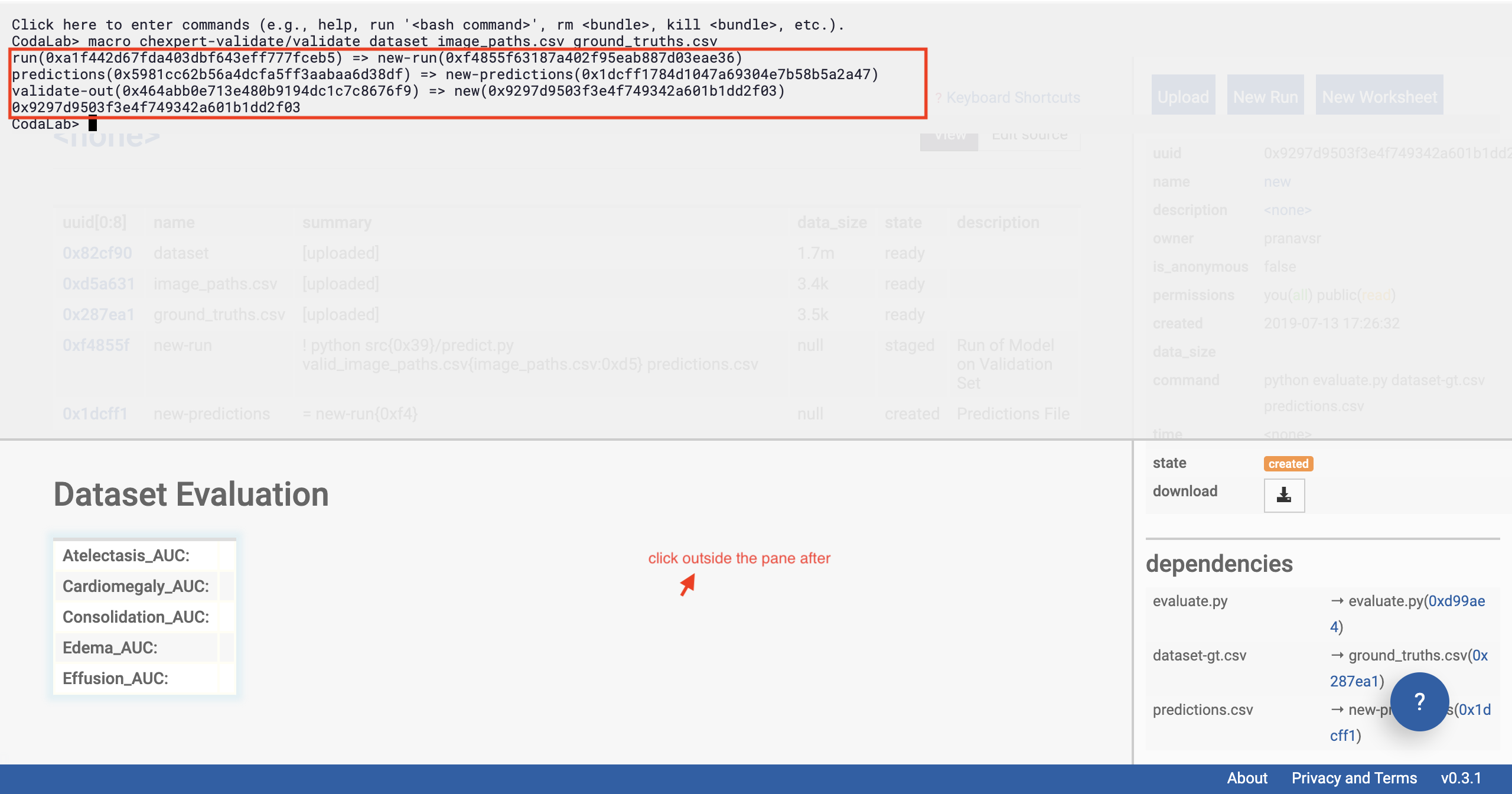 See the outputs and click outside
You should be able to see that Dataset Evaluation and a few rows have been added to the table on the left of the page.
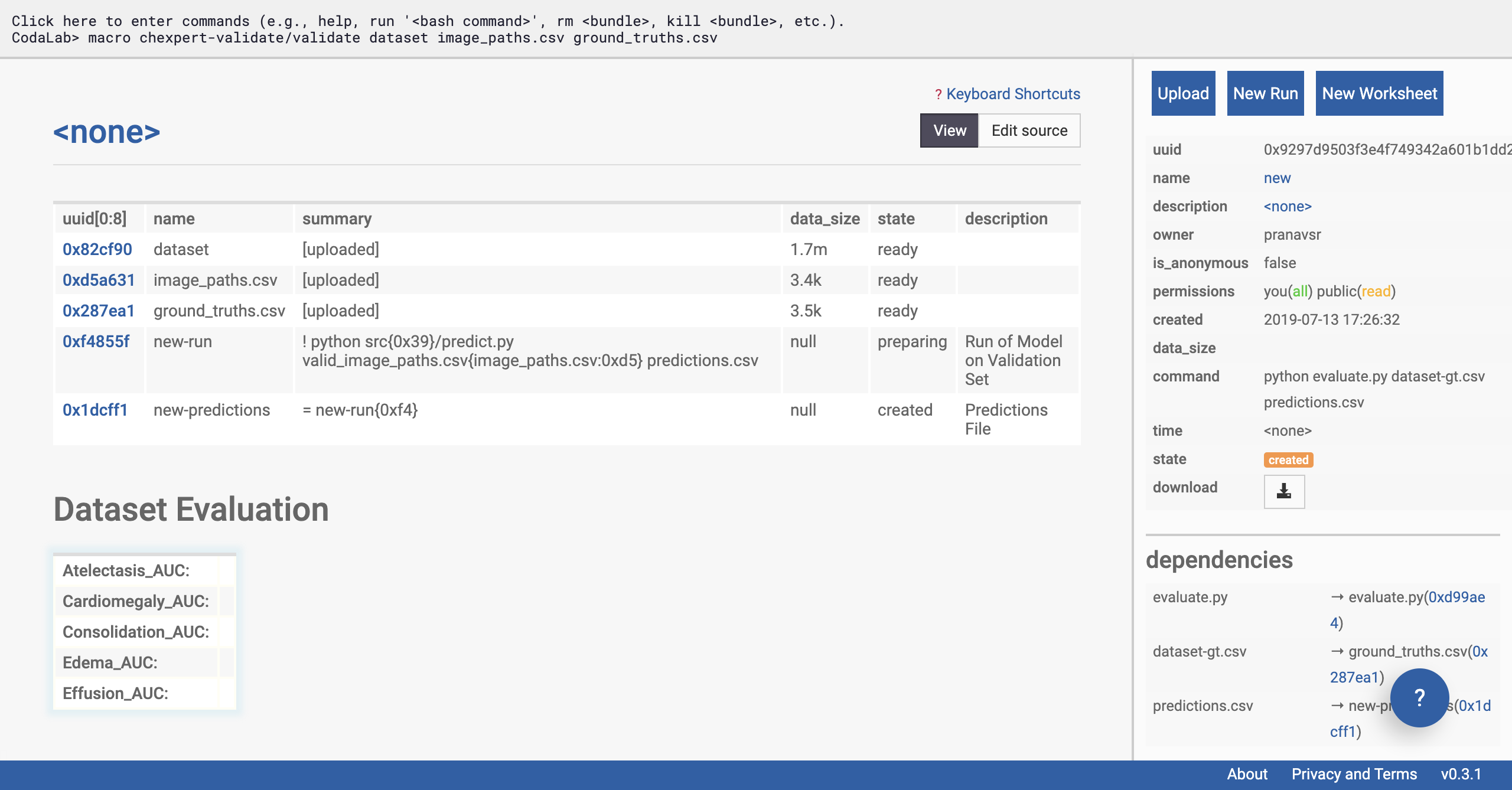 Verify that a few files are appended to your worksheet
Click on the ‘new-run’ row of the table on the left side of the page (see selection in figure below). The sidebar should change, and now display information about the status of the model’s run on the data.
We’re going to give special attention to the ‘state’ of the run. This will start with ‘preparing’, and can take a few minutes as the remote machine downloads the CheXpert models.
If your run goes to the ‘staged’ state, it means that the bundle is ready to run but it is waiting for appropriate resources to free up. CodaLab has a limited set of machines available (they’re free!), so when there are a lot of people wanting to run jobs, you might have to wait a long time. You can check out the Codalab status page to see where your jobs are in the queue (note that this page only sees public jobs, so there might be hidden bundles in the queue that you can’t see). If
you’d like to run your job earlier, you can easily attach your own compute workers, which you might want to do anyway if you have fancier GPUs, say.
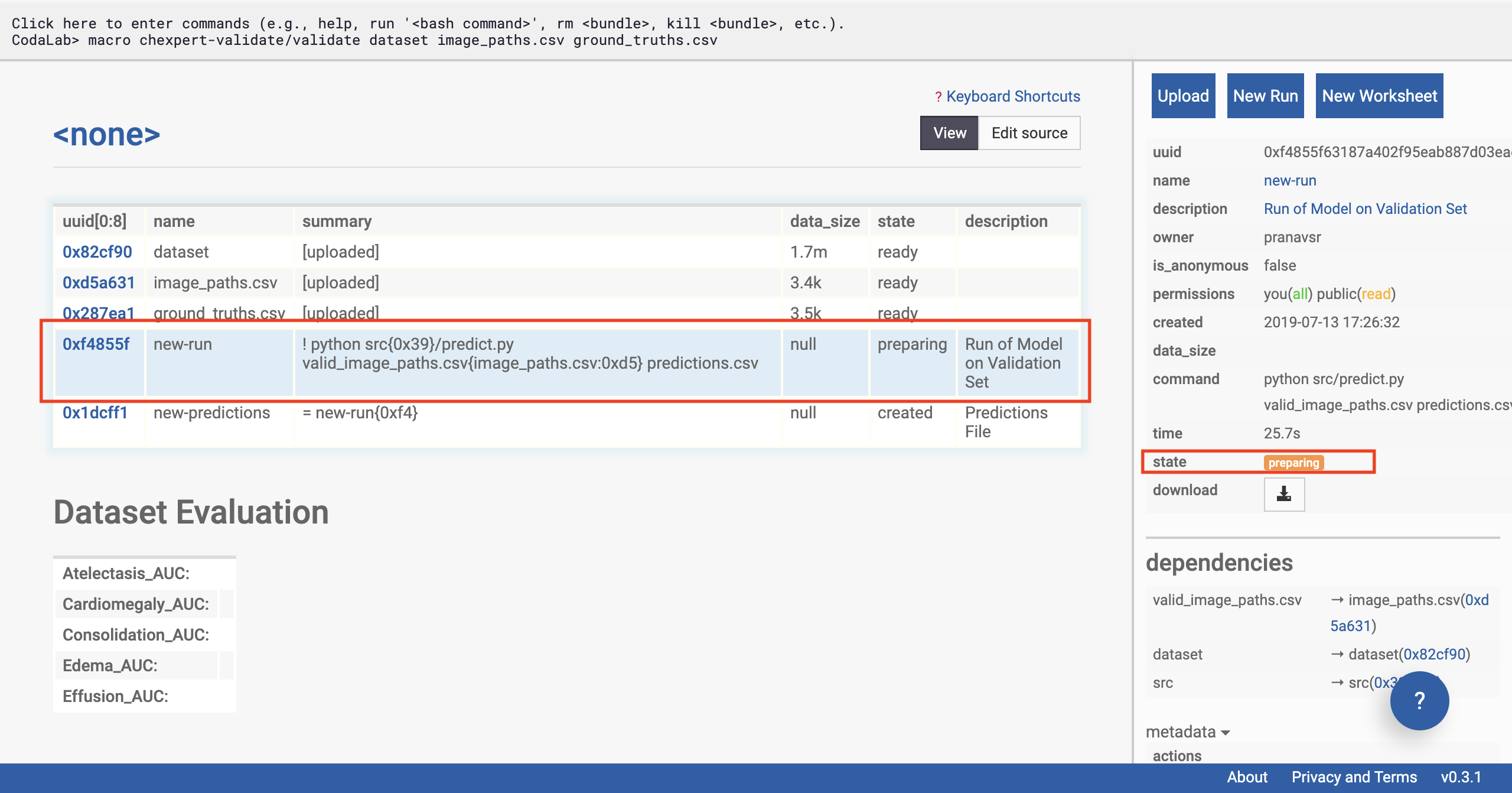 Check the status
Soon, the status of the run should update to ‘running’. Now the model has been loaded on to a machine, and predictions are being made on the uploaded dataset. This takes 10 minutes for us using the example dataset, and will take longer on a larger dataset. Note that the Chexpert model is not one model, but a collection of 30 specialist models, which must each be sequentially run on the data.
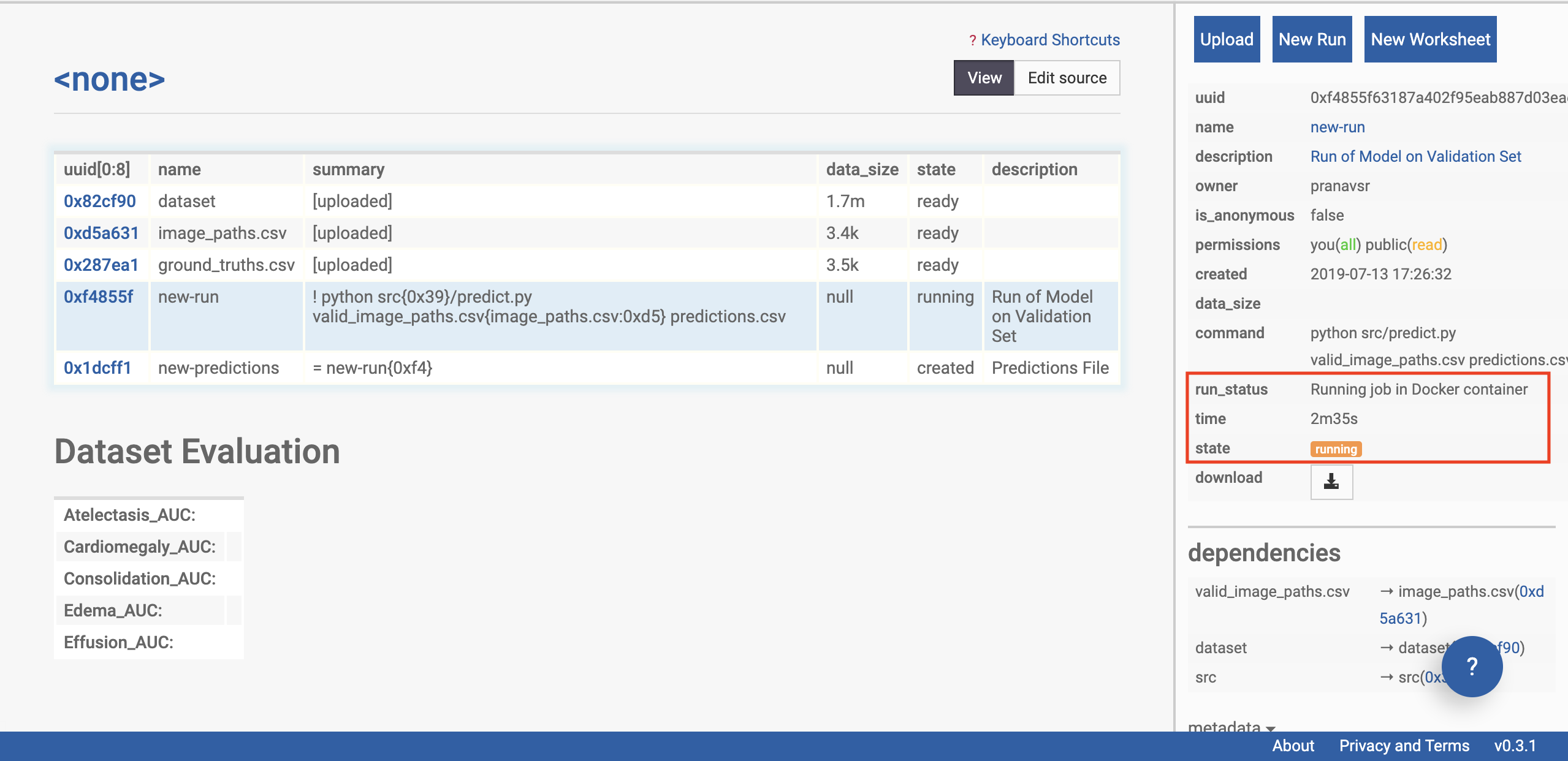 Check the status again
Once the model has finished running, the status of the run will update to ‘ready’. In a few seconds, the table should auto-populate (refresh the page if it doesn’t) with the AUC scores of the model on the data across the various tasks (using the ground truth you’ve supplied).
If you see an error, please go back to the previous steps, and make sure that you haven’t missed any instructions.
Optional: if you’re an advanced user looking for confidence intervals on the AUC or further statistical analysis, advanced users can download the prediction file by clicking on the ‘new_predictions’ row, and then clicking download on the sidebar.
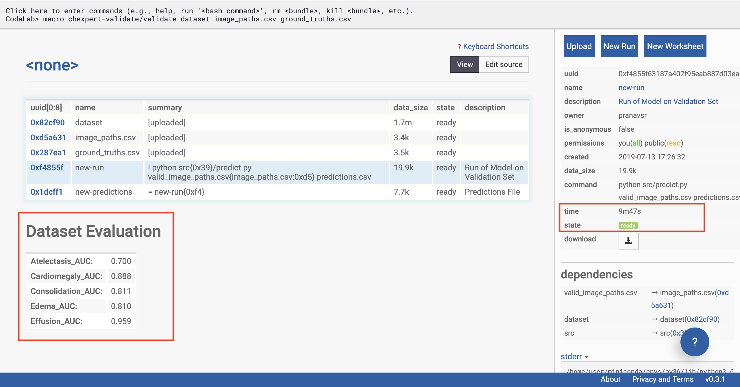 Running is completed
And that’s it! You’ve just validated the CheXpert model on your own data (or the example data)!
Join us in a worldwide effort
If you’ve followed our tutorial and successfully validated CheXpert model on your own institution’s data (or data that’s not from our google image example), we’d love to know! Please let us know how CheXpert did on your population! We encourage you to publish, and to also join our efforts in compiling the performances of the model on data worldwide. Email us at:
Acknowledgements
Thanks to our colleagues Nguyet Minh Phu and Mark Sabini for collecting and labeling the google images dataset we use in our example. Thank you to Amit Schechter, Anuj Pareek MD, and Evan Zucker MD for testing and timing the walkthrough.